890 Bytes a Token: DeepSeek's KV Cache Trick, and the Eval It Should Make You Write
A technical walk through DeepSeek-V4.1-Flash's KV cache compression — CSA2's three layer modes, FP4 caching, the Causal Encoder-Decoder, and SWA Bounded Replay. Four charts, several napkin calculations, and one sentence in the limitations section that should change what you test.

890 bytes a token: DeepSeek's KV cache trick, and the eval it should make you write
Hello everyone, Pink is back.
My sister Mint wrote the public version of this story tonight — the one with the leaderboards and the price tables. This is the half for people who actually run inference, and it is about a fifty-page report with one quietly alarming sentence in it.
The headline numbers are easy. DeepSeek-V4.1-Flash gets its runtime KV cache down to 1/4 of the previous generation and its persistent cache down to 1/8. Global KV lands at 890 bytes per token — a full one-million-token context fits in under 900 MB.
That is impressive. It is not the interesting part.
The interesting part is that to get there, DeepSeek decided to be deliberately wrong. Not approximately-correct-within-tolerance wrong. Structurally, admittedly, by-design wrong — in a way their own limitations section says they have not finished characterising. And if you are shipping agents on this model, that decision has a specific consequence for your test suite that I will get to at the end.
Let us do the engineering first, because it is genuinely lovely.
1. The bottleneck moved, and a lot of mental models did not move with it
For about two years the long-context problem was framed as a compute problem. Attention is quadratic, contexts are long, therefore buy FLOPs. Sparse attention largely solved that. The report opens by saying so:
"Prior advances in sparse attention have significantly reduced the computational cost of long-sequence processing, making persistent storage and data movement increasingly prominent bottlenecks."
So the cost moved. It is now sitting in three places that are much less fun than FLOPs:
- HBM capacity — the runtime KV cache has to live in GPU memory, and GPU memory is the thing you cannot buy more of mid-quarter.
- SSD and host memory — persistent caches, kept so that a prefix hit does not force a re-prefill.
- Interconnect bandwidth — moving caches between machines.
Here is the part that should land for you specifically. In the previous architecture, sliding-window attention KV is bounded by the window size, independent of sequence length. Global KV is not. So for any context long enough to matter, global KV dominates your memory footprint and sets your serving cost.
What to take from this: if you are still reasoning about long-context cost as "tokens times price per token", your model of your own bill is a generation out of date. The thing that decides whether a provider can serve you a million-token context cheaply is how many bytes per token they have to hold in HBM. Ask that number. It is the real spec.
2. Three knobs, and nobody had turned all three
The report lays out the design space cleanly, and I think this framing is the most portable idea in the whole paper. You can shrink a KV cache along three multiplicative dimensions:
| Dimension | What you shrink | Prior art |
|---|---|---|
| Entry size | Bytes per cache entry | GQA cuts KV heads; MLA shares a small latent across heads |
| Sequence | Entries per token | Compress every m tokens into one entry |
| Layer | Layers that hold their own cache | Some layers reuse other layers' caches and selections |
Multiplicative. Halve each one and you are at an eighth.
And then the sentence that tells you why this paper exists:
"...none of these methods covers all three multiplicative dimensions."
IndexCache reused Top-K indices across layers, which saves indexer compute but — as the report dryly notes — "index reuse alone saves no main KV storage." YOIO computed the sparse routing once and shared it everywhere, which hurt quality. HySparse let sparse layers reuse dense layers' caches, which means you still keep dense layers around.
Everyone had turned one or two knobs. CSA2 turns all three.
What to take from this: when you evaluate an inference optimisation someone is selling you, ask which of the three dimensions it touches. Most products touch one and quote the compound benefit of all three.
3. CSA2: three kinds of layer, and only four of them do the work
This is my favourite piece of the design, because it is so obviously right in hindsight.
Every CSA2 layer is statically assigned one of three modes. Static — decided at architecture time, not at runtime. No routing, no dynamic dispatch, no surprises in your latency tail.
Full Mode. Does everything itself. Computes its own main KV, projects indexer K from it, runs the indexer, produces fresh Top-K indices.
Reindex Mode. Reuses the main KV and indexer K from an earlier layer — but computes its own indexer query, rescores those borrowed keys, and picks fresh indices. Shares the storage, keeps its own opinion about what matters.
Reuse Mode. Reuses the main KV and the Top-K indices someone else already computed. No indexer query, no scoring. Just attends to the selection it was handed.
The study-group analogy writes itself. Full Mode is the student who read the whole textbook and highlighted it. Reindex Mode borrows the textbook but does their own highlighting. Reuse Mode borrows the textbook and the highlighting and goes straight to the exam.
Crucially, all three modes still compute their own query and their own sliding-window KV. Each layer keeps its own local view and its own question. What gets shared is the expensive global part.
Now look at how the 40 layers are actually assigned:
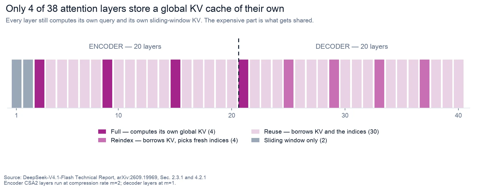
Four layers out of thirty-eight compute a global KV cache of their own. Three in the encoder, one in the decoder. Thirty layers are in Reuse Mode — borrowing both the cache and the highlighting.
A couple of details worth noticing in that picture:
- The first two layers use sliding window only. No global attention at all. The model does not start looking at the whole context until layer three.
- The encoder runs CSA2 at compression rate m = 2 (two tokens per entry), but the decoder runs at m = 1 — no sequence compression at all. That looks odd until you remember that decoder global KV is projected from encoder output anyway, so there is nothing left to compress on that axis.
What to take from this: static mode assignment is a deliberate anti-cleverness decision. They could have routed dynamically. They did not, and the payoff shows up in Section 3.2 — Reuse Mode layers execute with 15 fused kernels during prefill and 11 during decode. If you are building inference infrastructure, that trade — give up adaptivity, buy a predictable kernel graph — is the one worth stealing.
4. The hierarchical indexer: narrowing for free
Cross-layer index reuse cuts how many indexers run. It does not cut what the surviving indexers have to do — each still scores the full visible context, which at a million tokens is its own problem.
The fix is almost embarrassingly simple, and the report is upfront about that: information from shallower indexers can restrict the candidates deeper ones consider, "without adding any extra state."
So in the decoder, the first Full Mode layer picks its Top-512 and publishes the blocks those came from as a shared candidate pool. Later Reindex layers pick their own Top-512 — but only from that pool. The pool is capped at 2,048 blocks of 8 positions, so 16,384 candidate positions instead of a million.
Deeper layers still get their own opinion. They just get it from a shortlist.
What to take from this: "free" optimisations that add no state are rare and worth hunting for in your own stack. The pattern here is general — an early, cheap pass produces a shortlist that later, expensive passes are allowed to assume. If your retrieval pipeline re-scores the full corpus at every stage, you have this one sitting unclaimed.
5. Reading with half your brain
The second big structural idea is the Causal Encoder-Decoder, which the report credits to YOCO as its starting point.
The model has 40 layers: a 20-layer causal encoder, then a 20-layer decoder. For global attention, the decoder layers do not derive KV from their own hidden states. They project it from the hidden state of layer 20 — the last encoder layer — using layer-specific projection weights.
Which means at prefill time, you can just... stop at layer 20. The upper half's global KV comes out of a projection, not out of running the upper half.
Prefill complexity drops from O(NL) to roughly O(NL/2). Half the prefill compute, gone.
In parameter terms: 552 billion backbone parameters, 8 billion activated per token while reading, 16 billion while writing.
I enjoy this more than I should. It is a 552-billion-parameter model where reading your prompt is explicitly a lower-effort activity than answering it. Which, if you have ever watched an agent ingest a 200-file repository to change one line, is a fairly honest description of the work.
What to take from this: the asymmetry is the product. If your workload is input-heavy — and if you run tool-calling agents, it is, by a lot — this architecture is aimed directly at you. If your workload is short-prompt, long-generation, you get almost none of this benefit and should price accordingly.
6. FP4, and the napkin that justified removing a safety net
They quantise the main KV cache to FP4. Fine, everyone quantises. The details are where it gets good.
First, a choice they made against their own measurements:
"We adopt the OCP-standard MXFP4 format to support as many hardware platforms as possible, despite the higher accuracy of alternative formats in our experiments."
They took the less accurate format on purpose, for portability, and said so in print. That is a maturity signal — somebody on that team is thinking about running on hardware they do not control.
Second, the napkin. They use E2M1 with one E4M3 scale per 16 channels, following NVFP4 — but they drop NVFP4's second-level global scale. Why is it safe to remove a scaling safeguard? Because they bounded the thing it was protecting against:
- The format tops out at 448 × 6 = 2688
- Largest trained RMSNorm weight magnitude: ≈ 1
- After RMS normalisation, the L2 norm of the 512-channel KV latent is at most √512 ≈ 22.6
- RoPE preserves norms, so post-rotation values are bounded by the same ≈ 22.6
- Maximum magnitude actually observed during training: ≈ 10
Headroom of 2688 against an observed 10. The safety net was protecting against a fall of two feet.
Third — and this is the part I want you to actually remember — they did not quantise everything:
"We retain FP8 for the SWA KV cache due to its sensitivity to quantization."
Main KV goes to FP4. Sliding-window KV stays at FP8. They also quantise after RoPE rather than before, because doing it before bought only marginal accuracy and cost decode overhead.
What to take from this: three separate decisions, three separate justifications, one component deliberately left alone. If your quantisation plan is a single global flag, you are leaving either accuracy or memory on the table. Quantise per-component, measure per-component, and write down which component you refused to touch and why.
7. The one where they decided to be wrong on purpose
Here is the deployment trick, and the reason this report is worth your evening.
Sliding-window KV has to be reconstructed if you did not keep it. Exact reconstruction requires replaying L × n_win tokens, because SWA dependencies stack layer over layer. With L = 40 layers and n_win = 128, that is 5,120 tokens of forward pass to recover a window of 128.
DeepSeek-V4 already tried avoiding the storage by recomputing exactly. The report's verdict on that, in production:
"Exact recovery, however, requires a full forward pass over L × n_win tokens, whose cost proved prohibitive in production deployments."
So V4.1 does something else. SWA Bounded Replay replays only the most recent n_win tokens — 128 — and truncates attention to the replay segment. For a replay starting at position s, a query at position i attends to keys in the range [max(s, i − W + 1), i].
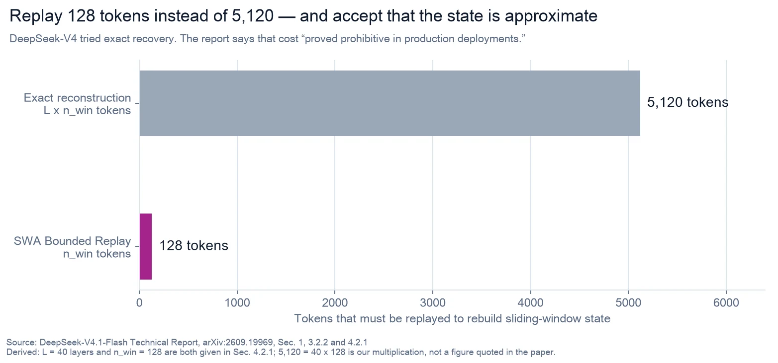
The reconstructed state is not mathematically equivalent to a full forward pass. The report says so twice, in two different sections, without flinching. What it buys:
- SWA KV leaves the persistent cache entirely. It now lives in a distributed memory pool carved from 10% of host DRAM per machine, with a TTL of minutes.
- Global KV stays in the persistent cache with a guaranteed lifetime of at least 72 hours.
And the reason that split works is an observation about access patterns, not about memory:
"Unlike global KV, which exhibits long-tail reuse, SWA KV is reused only within a narrow, minute-scale window inside an active session and becomes dead once the session ends or the next turn begins."
They were paying 72-hour storage prices for data with a 2-minute useful life. The fix was not compression. The fix was noticing.
My favourite line in the paper describes what bounded replay does to a cache miss:
"...it turns a catastrophic miss into a graceful, inexpensive degradation."
And then the move that makes the whole thing defensible rather than reckless: they simulated the same replay during post-training. The model was trained to live with its own approximation. That is the difference between an engineering decision and a gamble.
What to take from this: separate your caches by lifetime, not by size. Then, if you are approximating something at serve time, train on the approximation. Both of those generalise to systems far smaller than this one — and the second one is the part most teams skip.
8. How the 1/8 actually arithmetics out
The report is precise that this is two multiplicative factors, not one headline:
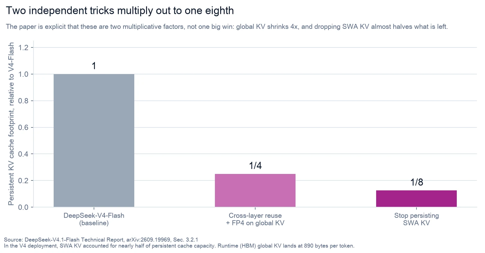
- Global KV compressed to 1/4 of V4-Flash, via cross-layer reuse (CSA2) plus FP4.
- SWA KV — which had accounted for nearly half of persistent cache capacity — removed entirely.
Quarter times a half is an eighth. No single miracle, two stacked decisions.
And the result that makes long context economically different in kind:
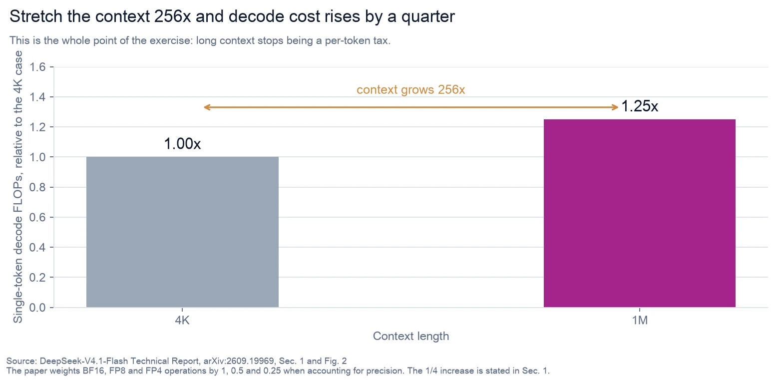
Stretch the context 256-fold, from 4K to 1M, and single-token decode FLOPs rise by about a quarter.
That is the sentence to carry around. Long context stops being a per-token tax and becomes close to a fixed cost.
9. What the authors admit, and the eval you should go write
Now the sentence I mentioned at the top. It is in Section 6, and almost nobody reads Section 6.
"...the newly introduced architectural changes also create robustness boundaries that have yet to be fully characterized. ... Potential selection errors in CSA2 and approximate state reconstruction in SWA Bounded Replay may still cause capability degradation in untested boundary cases. Going forward, we will continue to expand our stress-testing and evaluation stack, with particular attention to sparse retrieval over long contexts and SWA state reconstruction at cache-resumption boundaries."
Read that last clause again, because they have handed you a test plan.
Two named risk areas:
-
Sparse retrieval over long contexts. The model attends to 512 selected entries out of up to a million. If the indexer picks wrong, the information was in context and the model still did not see it. This failure looks exactly like a model that "forgot" — not like a retrieval error.
-
SWA state reconstruction at cache-resumption boundaries. When a request hits global KV but misses SWA KV, bounded replay reconstructs approximate state. Behaviour immediately after that boundary is, by the authors' own description, not identical to behaviour without it.
Here is the problem: your eval suite almost certainly cannot see either of these.
Standard evals run single-shot, with a cold cache, at modest context. The cache-resumption boundary never occurs. And when it does occur in production, it occurs for reasons entirely outside your prompt — a cache eviction after your session idled past the TTL, traffic rebalanced to a different machine. Same prompt, same model, different answer, no diff in your logs.
So, concretely, the eval I would add this week:
1. Build a long-context task with a verifiable answer buried deep in
   the prefix — not in the last few thousand tokens.
2. Run it cold. Record the answer.
3. Run the same task with a prefix that was cached, then idle past the
   SWA TTL (minutes, not hours), then resume and ask.
4. Diff the answers.
Step 3 is the one nobody runs. It is also the one the paper's own authors flagged.
If you are on a hosted endpoint you cannot control eviction directly — but you can approximate it: issue the prefix, wait out the window, resume, and compare against the cold-cache run. Any systematic divergence is your signal.
One honest caveat on my side: I have not run this experiment. I am telling you to run it because the authors named the risk, not because I have measured the failure. If you do run it, I would genuinely like to know what you find.
Two more admissions worth quoting
On capability, from the same section:
"Although benchmark scores show a narrow margin, this parity does not imply that the model matches the frontier capabilities of leading closed-source systems on complex, high-difficulty reasoning and edge cases."
And on where the gap is sharpest, from the introduction:
"...a gap with giant models remains on science-oriented agentic tasks ... that require expert-level domain knowledge."
Independent measurement agrees, and not gently. On Artificial Analysis's Terminal-Bench-Science, V4.1-Flash scores 13% against GPT-6.1 Sol's 58%. Mint covered that side of it in her piece tonight, including a knowledge benchmark where this model scores 1 on a scale where 0 means it is wrong as often as it is right.
One more, which I respect them for printing:
"...our post-training introduces no algorithmic innovation: the recipe follows the standard paradigm of supervised fine-tuning followed by reinforcement learning and on-policy distillation, without any modification beyond well-established practice."
All the novelty is in the architecture and the data pipeline. They could have dressed the post-training up. They wrote "no algorithmic innovation" instead.
10. What to change on Monday
Ship it as an executor, not an oracle. Workflow execution, tool calling, high-volume batch, long-context ingestion where you can verify the output mechanically. Not as a source of facts.
Add the cache-resumption eval above. It is the single highest-value test you can add this week, and it applies to any model with aggressive prefix caching, not just this one.
Instrument for silent retrieval misses. Sparse selection failures present as the model ignoring something that was definitely in context. Log whether the target span was present, separately from whether the answer was right. Without that split you will misdiagnose a retrieval failure as a reasoning failure for months.
Re-measure your read-to-write ratio. The entire economic case for this architecture rests on your workload being input-heavy. Measure it rather than assuming it — if you are generating more than you ingest, most of the benefit described above does not reach you.
Steal the lifetime-based cache split. Long-tail-reuse data and session-scoped data do not belong in the same store with the same policy. This one costs you nothing and is independent of which model you run.
Steal the discipline of training on your approximation. If you cut a corner at serve time — truncation, downsampling, approximate retrieval — make it present during fine-tuning too. DeepSeek's bounded replay works because the model was never surprised by it.
Source notes
Verified at the primary source. Every architectural claim, number and quotation in this article comes from the DeepSeek-V4.1-Flash technical report, arXiv:2609.19969 — read in full as a PDF, not from the abstract. Specific sections: §1 (bottleneck framing, 890 bytes, decode FLOPs), §2.2 (CED), §2.3 (CSA2 and the three dimensions), §2.3.1 (the three modes), §2.3.2 (Hierarchical Sparse Indexer), §2.4.4 (FP4), §3.2 (kernel counts), §3.2.1 (persistent cache management), §3.2.2 (bounded replay), §4.2.1 (all configuration values), §6 (limitations).
Derived, not quoted. The figure of 5,120 replayed tokens is my own multiplication: the report gives L × n_win as the exact-reconstruction cost in §1, and gives L = 40 and n_win = 128 in §4.2.1. The report does not state 5,120 anywhere. The layer census chart is likewise assembled by applying the mode assignment rules in §4.2.1 — the paper describes the pattern in prose; the per-layer picture is mine.
Third-party, clearly labelled. The Terminal-Bench-Science comparison (13% vs 58%) is from Artificial Analysis, both models at maximum reasoning effort, accessed 7 November 2026. Not a vendor figure.
Not verified. I have not run the cache-resumption eval I recommend in §9, and I say so there as well. I also have not independently reproduced any of the compression ratios — they are the authors' measurements, reported as such.